TL;DR
A spatial join links two datasets by location rather than a shared reference, a buffer draws a zone at a set distance around something, and an overlay cuts one layer by another. Chained together they answer most site, risk and proximity questions. Most wrong answers come from double counting in joins, distances measured in the wrong units, broken shapes and area figures that were never recalculated.
Once you understand vector vs raster data, the next question is what you can do with it. Most of the questions organisations bring to GIS are about where things are: which of our properties sit in a flood zone, which sites are within reach of a substation, how much of this land is left once the protected areas are taken out. Spatial joins, buffers and overlays answer nearly all of them. Each is simple to run, and each has a habit that can change the answer without any warning, which is worth knowing whether you run the analysis yourself or are handed the results.
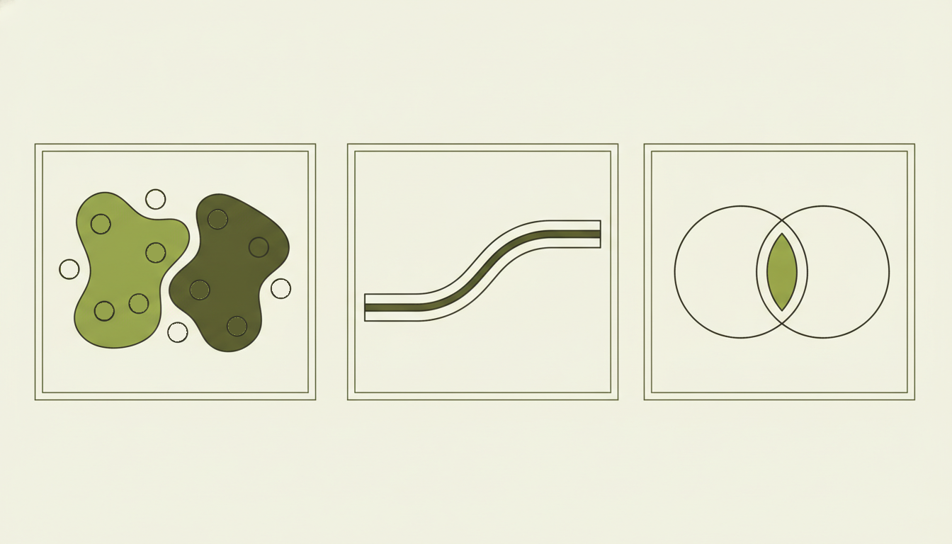
Left to right: a spatial join gives each point the details of the area it falls in, with points outside both areas left unmatched; a buffer draws a zone at a set distance around a line; and an intersect keeps only the area two layers share.
Spatial join: matching data by location
An ordinary join links two tables through a value they share, such as a customer number. A spatial join links them through location instead. Say you hold a list of 5,000 residential properties with no flood information, and the Environment Agency’s flood zones as a map layer. Nothing in the two datasets matches by reference number; the only thing they share is where they are. A spatial join tags each property with the flood zone it falls in, and the result is an ordinary table you can filter, count and report on.
The join needs a rule for what counts as a match. The usual one is “intersects”, meaning the two features touch or overlap at all, which suits a question such as whether any part of a site sits in a flood zone. “Within” is stricter and only counts a feature lying wholly inside another, which suits points inside council boundaries. “Nearest” matches each feature to the closest one in the other layer, such as the nearest substation or railway station. In QGIS these sit in the Join attributes by location and Join attributes by nearest tools.1
Choosing the rule is part of the analysis, and it changes the result. A site that clips the edge of Flood Zone 3 counts as in the zone under intersects but not under within, so a report built on one rule will disagree with a report built on the other.
The behaviour that catches most people out is that a spatial join can give you more rows than you started with. If a property straddles the boundary between Flood Zone 2 and Flood Zone 3, it matches both, so it appears twice in the output. Add up the floor area or the asset value from that table and the property has been counted twice.
QGIS makes the choice explicit: keep a separate row for each match, keep only the first match, or keep the match with the largest overlap.1 The first match is arbitrary and rarely what you want for reporting. The largest overlap is defensible, although it hides the fact that part of the site sits in the higher-risk zone. For a flood screen we would usually keep every match and then report the worst zone for each property. That works because the zones are ordered: Flood Zone 3 is land with a 1% or greater annual chance of flooding from rivers, or 0.5% or greater from the sea, and Flood Zone 2 covers the band below that down to 0.1%.2 The highest zone a property touches is therefore a fair summary of its exposure.
Buffer: drawing a zone around something
A buffer draws a new shape covering everything within a set distance of a feature. Buffer a river by 8 metres and you get a strip either side of it; buffer a substation by 2 kilometres and you get a circle standing in for a plausible connection distance. On its own a buffer answers nothing, since its job is to create the zone that the next step, usually a join or an overlay, needs.
A buffer distance is measured in whatever units the data’s coordinate system uses.3 Most UK data is in British National Grid, where the units are metres, so a buffer of 500 means 500 metres. Data in latitude and longitude, which is how GPS devices and many web sources supply it, uses degrees instead, and a buffer of 500 degrees covers the whole planet. A buffer that looks sensible in degrees is still wrong, because a degree of longitude is much shorter in Essex than at the equator, so the circle comes out as an oval on the ground. Our post on map projections explains why. The fix is to convert everything into one metre-based system before measuring anything.
Buffers around neighbouring features overlap. Buffer 40 listed buildings in a town centre by 50 metres and you get 40 overlapping circles, so any area calculated from them counts the overlaps more than once. Merging them into one shape, which GIS tools call dissolving, gives a single footprint with a true area.4
Sometimes you do not need the shape at all. “Which of our sites are within 2 kilometres of a substation?” can be answered with a straight distance check, without drawing anything, and on large datasets that is much faster. Draw the buffer when you need it on a map or for a later step.
Overlay: cutting one layer by another
A spatial join copies information between layers but leaves the shapes alone. An overlay changes the shapes, cutting features where layers cross so that you can measure what lies where. The common forms are:
| Overlay | What you keep | Typical use |
|---|---|---|
| Intersect | Only the area in both layers, with information from both | Which part of each field is Grade 3a land |
| Clip | The part of one layer inside another, with its own information only | Trimming national data to a study area |
| Erase | The part of one layer outside another | Removing protected land from candidate sites |
| Union | Everything from both layers, split where they overlap | Combining two constraint layers into one map |
QGIS and ArcGIS Pro both document these tools, although the names vary slightly; QGIS calls erase Difference, for example.5,6
Clip and intersect are the pair most often confused, and the difference matters for reporting. Clip trims the shapes but leaves the attribute table exactly as it was,5 so an area or length stored in the table still describes the original, uncut feature. A field clipped down to a third of its size can go on reporting its full original area. That stale figure is one of the errors we find most often in data that has passed through several hands.
A worked example: screening land for solar
An early-stage solar screen uses all three. Start with land parcels. Buffer the hard constraints, such as watercourses, listed buildings and ancient woodland, add Flood Zone 3, and merge the lot into one constraint layer. Erase that from the parcels so that only unconstrained land remains. Intersect what is left with the agricultural land classification, so each remaining piece carries its grade, then join each piece to its nearest substation to give it a connection distance.
The output is a table of parcels with developable hectares, land grade and distance to the grid. That is the start of a shortlist rather than the end of one, because the softer criteria still have to be weighed, but it turns a county of land into something a team can review. Our post on renewable energy site selection covers the constraints themselves in more detail.
What to check when someone shows you a GIS result
You do not need to run the analysis to question it. These are the checks we make on any result built from joins, buffers and overlays, and each can be asked of whoever produced the work.
- Do the totals add up? If the number of properties, hectares or pounds is higher than the source data allows, a join that matched some features more than once is the likely cause. Ask how features matching more than one zone were handled.
- What units were the distances in? Ask which coordinate system the analysis used. Desktop GIS lines layers up on screen even when they are stored in different systems, so two layers can look perfectly aligned whilst a measurement mixes metres and degrees. The answer should be a single metre-based system, which for UK work is usually British National Grid.
- Were the shapes checked before the overlay? Boundaries that cross over themselves, often a product of hand digitising, make overlays fail or produce wrong areas. GIS tools can check and repair them before analysis,4 and that should be a standard step rather than a fix applied after something breaks.
- Are there slivers along shared edges? When two layers share a boundary that was drawn separately, an overlay produces thin slivers along the edge where the lines do not quite agree. They inflate feature counts and can make tiny areas look significant. Ask whether a minimum area was applied, or the layers were snapped together first.
- Were areas recalculated after cutting? After a clip or an intersect, any stored area or length needs recalculating. If the area column looks identical before and after, it probably was not updated.
- How long did it take to run? Speed is not a measure of quality, but a join that takes hours usually means the data has no spatial index, the lookup that lets GIS skip features nowhere near each other. Without one, joining two tables of 10,000 records each takes 100,000,000 comparisons.7 It suggests the data is set up for one-off use rather than repeated analysis, which is worth knowing if the same question will be asked every quarter.
What these tools answer
The questions that drive decisions in property, planning and energy are usually some form of “where does this fall?” or “what is left once the constraints are removed?”, and joins, buffers and overlays answer both. Knowing how they behave, particularly the double counting and the units, is enough to follow most GIS analysis presented to you and to ask the right question when a number looks wrong.
For an example of this kind of logic built into a working tool, see our solar site selection case study. The energy and renewables page covers how we work with developers, GIS project delivery covers defined pieces of analysis for teams without in-house GIS, and the Knowledge Hub has more introductory guides.
If you want to know how well your own spatial data would stand up to this kind of analysis, the GIS scorecard takes a few minutes and shows where the gaps are.
References
- QGIS documentation. Vector general.
- GOV.UK. Flood risk and coastal change, Table 1: Flood Zones.
- PostGIS documentation. ST_Buffer.
- QGIS documentation. Vector geometry.
- QGIS documentation. Vector overlay.
- Esri ArcGIS Pro documentation. Erase.
- PostGIS workshop. Spatial indexing.