Renewable energy site selection with GIS: how the constraint analysis actually works

The spatial logic behind renewable energy site selection is consistent across technologies. Build a constraint model, layer your datasets, run your exclusions, score what remains. The methodology does not change much whether you are looking at solar, onshore wind, or battery storage.

The constraint layers do.

Understanding where the datasets diverge by technology is where GIS analysis earns its keep. A constraint model built for a solar portfolio is not the right starting point for a wind assessment. The assumptions are different, the data sources are different, and some of the hardest constraints do not appear in the other technology’s workflow at all.

The shared spatial logic

Whatever the technology, constraint mapping starts from the same premise. You have a study area, a set of exclusion criteria, and a ranked shortlist at the end. The process splits into two passes.

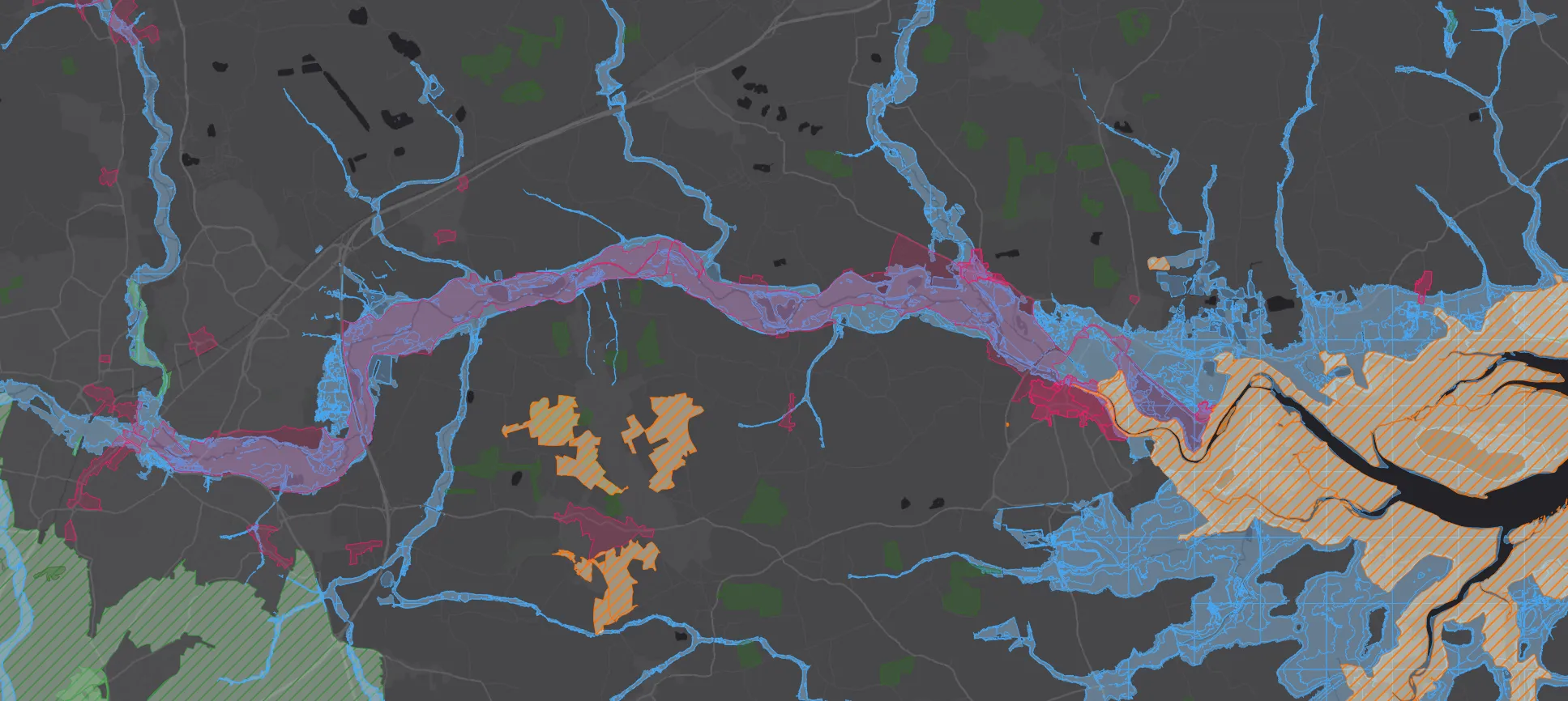
The first is binary exclusion. Every hard constraint becomes a yes/no mask. Land within a Site of Special Scientific Interest is out. Land in Flood Zone 3b is out. Overlap every exclusion layer and what survives becomes your search area. This is fast and effective for clearing unsuitable land early.

The second pass is weighted scoring. Instead of a hard cut, each factor is scored and weighted against project priorities. A site 500 metres from a substation scores higher than one 5 kilometres away. Grade 3b agricultural land scores higher than 3a. Run that model across your study area and you get a composite suitability ranking for every parcel.

Most assessments use both. Binary exclusion to set the boundary, weighted scoring to order what is left.

Where solar and wind diverge

Solar and wind share several constraint categories: environmental designations, flood risk, grid proximity, and land ownership fragmentation all appear in both. But the layers that differentiate them are significant.

For solar, agricultural land classification carries heavy weight. Planning policy discourages development on Best and Most Versatile land (ALC grades 1, 2, and 3a). Topography matters too. Panels perform best on flat or gently south-facing ground; slopes above roughly 15 degrees increase mounting complexity and construction cost. The constraint footprint for solar is relatively contained, which means site assembly is often simpler.

For onshore wind, the constraint picture is more complex. Noise is a statutory consideration: most local authorities apply a noise limit at nearby receptors, typically expressed as a dB(A) threshold, which generates a setback buffer around residential properties. Shadow flicker from rotating blades introduces a separate proximity constraint at dwellings. Aviation and Ministry of Defence radar safeguarding zones can knock out large areas entirely. Turbines also have a significantly larger landscape sensitivity footprint than solar panels, which means visual impact assessment and Zone of Theoretical Visibility analysis carry more weight at the constraint screening stage.

The data sources behind the constraints

Every layer in a constraint model comes from a specific source, and knowing where to get authoritative data (rather than a stale copy someone downloaded two projects ago) is most of the groundwork.

Environmental designations (SSSIs, SACs, SPAs, ancient woodland, National Landscapes) come from Natural England’s MAGIC service, which is free and updated regularly. Flood risk uses the Environment Agency’s Flood Map for Planning, which distinguishes Flood Zones 2 and 3 and factors in the Environment Agency’s climate change allowances for long-lived infrastructure. Agricultural Land Classification comes from Natural England’s ALC dataset, though the published mapping is often at a coarse regional scale and site-specific ALC surveys are usually needed before a planning submission, not just at the initial screening stage.

Grid connection data is the hardest to keep current. Distribution Network Operators publish capacity heat maps and connection registers, but headroom changes as other projects in the queue progress or drop out, so a constraint model built on grid data from six months ago can already be wrong. Aviation and radar safeguarding zones come from the Ministry of Defence and the Civil Aviation Authority, and both maintain their own mapping services that need to be checked independently, not assumed to be static.

Historic England’s National Heritage List covers listed buildings, scheduled monuments, and registered parks and gardens, all of which carry their own setting and setback considerations that do not always show up as a simple buffer distance.

A worked example: screening a 50-hectare solar site

Take a hypothetical 50-hectare parcel in the East of England being screened for a ground-mounted solar array. The binary exclusion pass starts by overlaying the parcel against SSSI and SAC boundaries (clear), Flood Zone 3b (a 2-hectare strip along the eastern boundary is excluded), and existing rights of way (a public footpath crosses the northern third, which does not exclude the land but does constrain the array layout around it).

That leaves roughly 46 hectares of unconstrained land. The weighted scoring pass then layers in Agricultural Land Classification (most of the site is Grade 3b, which scores favourably against planning policy’s preference away from Best and Most Versatile land), slope (the site is largely flat, with a small rise in the southwest corner exceeding the 15-degree threshold where mounting costs increase), and grid proximity (a 33kV substation sits 1.2km from the site boundary, well within the range where connection costs remain proportionate to project value).

The output is not a single yes/no answer. It is a suitability surface across the 46 hectares, showing the strongest sub-areas for the array layout and flagging where secondary considerations (footpath buffer, slope, distance to substation) should shape the detailed design. That surface, not a spreadsheet of pass/fail flags, is what a developer actually needs to take into detailed design and the planning application.

Common mistakes in constraint modelling

The most common error is treating grid data as static. A model built once and reused across a portfolio without rechecking DNO capacity will confidently recommend sites that no longer have headroom, because another project further up the connection queue has consumed it.

The second is applying national thresholds without checking local variation. Noise limits, landscape sensitivity assessments, and BESS-specific policies are increasingly set at the local authority level, and a constraint model built against national guidance alone will miss local supplementary planning documents that add stricter requirements.

The third is skipping ground-truthing on the constraints that matter most to the eventual planning decision. ALC mapping at a regional scale is a reasonable screening tool, but a planning officer will expect a site-specific ALC survey before determining an application. Treating the desk-based constraint model as the final answer, rather than the tool that narrows the search before targeted, harder-to-scale checks, is where site selection projects lose time later in the process rather than saving it early on.

For an onshore wind assessment, the same site would be screened very differently. A single 150-metre-tip-height turbine on that same parcel would need to clear noise setbacks from the residential properties bordering the site, a shadow flicker assessment for any dwelling within roughly ten rotor diameters, and a Zone of Theoretical Visibility check against nearby designated landscapes. Where the solar assessment cleared 46 of 50 hectares, a wind assessment on the same land might rule out turbine positions across most of it once noise and shadow flicker setbacks are applied, leaving only a handful of viable turbine locations rather than an open development area. This is exactly why a constraint model built for solar cannot simply be relabelled for wind: the spatial logic is shared, but the usable outcome is not.

Battery storage: a different set of questions

Battery energy storage systems (BESS) have a different constraint profile again. They are largely insensitive to agricultural land quality and topography, which removes two of the biggest filters from the solar workflow.

The critical spatial questions for BESS are about infrastructure and safety. Proximity to high-voltage grid infrastructure is paramount: a BESS site needs to be close enough to a substation or grid connection point that the connection cost does not undermine the project economics. Fire safety separation from occupied buildings and transport corridors is increasingly formalised in planning guidance following incidents in the sector. Some local authorities have introduced specific BESS policies that add spatial constraints not present in the national framework.

BESS assessments also have to account for cumulative grid capacity in a way that is harder to model spatially. Available grid headroom is a moving target, which means the constraint analysis needs to be paired with live DNO data and capacity forecasting.

Why technology-specific models matter

It is tempting to start with a generic “renewable energy” constraint model and adapt it for each technology. In practice, that produces models that are either too conservative (applying solar constraints to wind assessments, for example) or that miss technology-specific hard constraints entirely.

The cleaner approach is to build the model for the technology and the study area from the start. The datasets are largely publicly available. The methodology is well-established. What takes time is the data preparation, the validation, and the judgement calls about how to weight competing factors for a specific project context.

You can see this approach in practice in our site selection case study — a working application delivered in three weeks for an energy developer, consolidating fragmented data into a structured constraint model their team could actually use. This kind of constraint modelling sits within our energy and renewables work, and the Knowledge Hub covers more of the underlying GIS terms and methods referenced above.

If you are working across a portfolio of renewable projects and want to bring structured GIS constraint analysis into your site assessment workflow, get in touch.